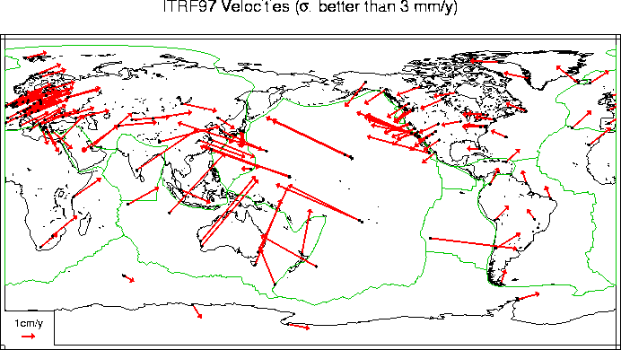
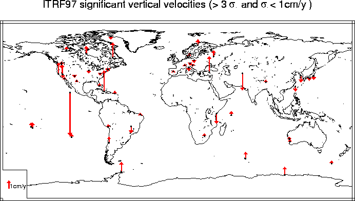
ITRF97
Input data
$$\global\def\fig#1{\scriptsize\textcolor{E83E8C}{fig.#1}}$$ $$\global\def\tab#1{\scriptsize\textcolor{E83E8C}{tab.#1}}$$
The individual solutions selected for the ITRF97 analysis are 4 VLBI, 5 SLR, 6 GPS, 3 DORIS and one multi-technique (SLR + DORIS) solution.
These solutions are summarized in $\tab1$.
On the other hand, the local ties of collocation sites, used in the ITRF97 adjustment were first converted into a complete set of positions for each site expressed in SINEX format.
| Solution | Data Span yy-yy |
Station nb. | Ref. Epoch y:doy |
|---|---|---|---|
| VLBI | |||
| SSC(GSFC) 98 R 01 | 79-98 | 129 | 97:001 |
| SSC(GIUB) 98 R 01 | 85-97 | 49 | 93:001 |
| SSC(NOAA) 95 R 01 | 79-94 | 107 | 93:001 |
| SSC(USNO) 98 R 01 | 79-98 | 110 | 97:001 |
| SLR | |||
| SSC(CGS) 98 L 01 | 86-98 | 76 | 93:001 |
| SSC(CSR) 98 L 01 | 76-98 | 129 | 93:001 |
| SSC(DUT) 98 L 01 | 83-97 | 72 | 93:001 |
| SSC(GSFC) 98 L 01 | 80-97 | 38 | 86:182 |
| SSC(GZ) 98 L 01 | 93-98 | 51 | 93:001 |
| GPS | |||
| SSC(CODE) 98 P 01 | 93-98 | 139 | 95:314 |
| SSC(EMR) 98 P 01 | 94-97 | 40 | 98:001 |
| SSC(EUR) 98 P 01 | 96-98 | 67 | 97:074 |
| SSC(GFZ) 98 P 01 | 93-97 | 76 | 97:001 |
| SSC(JPL) 98 P 02 | 91-98 | 84 | 96:001 |
| SSC(NRCAN)98 P 01 | 95-98 | 145 | 98:001 |
| DORIS | |||
| SSC(CSR) 96 D 01 | 93-96 | 54 | 93:001 |
| SSC(GRGS) 98 D 01 | 93-98 | 63 | 93:001 |
| SSC(IGN) 98 D 04 | 90-97 | 69 | 94:001 |
| Multi-technique | |||
| SSC(GRIM) 98 C 01 | 85-96 | 143 |
Data analysis
$$\global\def\fig#1{\scriptsize\textcolor{E83E8C}{fig.#1}}$$
The ITRF97 solution is derived with the following properties:
- All the individual matrices were orthogonaly projected using equation (3)
- Station positions of the projected solutions were then propagated at their epochs of Minimal Position Variance
- The reference frame definition (origin, scale, orientation and time evolution) is achieved in such a way that ITRF97 is in the same system as the ITRF96
- Station velocities are constrained to be the same for all points within each site
- ITRF97 positions were estimated at epoch 1997.0
- Transformation parameters (at epoch 1997.0) and their rates from ITRF97 to each individual solution were also estimated
Combination model
Assuming that for each individual solution $s$, and each point $i$, we have position $X^i_s$ at epoch ts and velocity $ \dot X^i_s $, expressed in a given TRF $k$.
The combination consists in estimating:
- Positions $X^i_{itrf}$ at a given epoch $t_0$ and velocities $\dot{X}^i_{itrf}$ in ITRS
- transformation parameters $T_k$ at an epoch $t_k$ and their rates $\dot T_k$, from the ITRF to each individual frame $k$
The general physical model used is given by the following equation :
where for each individual frame $k$, $D_k$ is the scale factor, Tk is the translation vector and $R_k$ is the rotation matrix. The dotted parameters designate their derivatives with respect to time.
Orthogonal projection
In some solutions and in particular those derived with 'free network' approach, the underlying reference system is loosely fixed and consequently this disturbs the quality assessment of the individual solutions included in the combination. For a given solution of positions and velocities, $X_s$, with its associated covariance matrix $\Sigma_s$, this latter contains both the natural observation noise and the RSE. The orthogonal projection consists in replacing, in $\Sigma_s$, the original RSE by a well known and small RSE, for all individual solutions to be combined together. This could be achieved by constructing an orthogonal projector $B$ as:
where:
- $A$ is the matrix of partial derivatives:
- ($x^0_i, y^0_i, z^0_i$) are the approximate coordinates of each point $i$
Using the orthogonal projector ($\fig2$), $\Sigma_s$ is modified by:
where $\theta$ is the vector of the transformation parameters; $\theta = (T_x, T_y, T_z, D, R_x, R_y, R_z, \dot{T}_x \dots)^T$ and $\Sigma_{\theta}$ is a diagonal matrix containing small variances for each transforamtion parameter.
Minimal Position Variance Investigation
It is usual to consider that the appropriate epoch to which station positions should be referred, is the 'central epoch' of the used observations. This is theoretically true if the observations are regular and have the same quality in time. On the other hand, if positions and velocities are solved for, together with full variance covariance between them, then the corresponding matrix should reflect the overall quality (or internal consistency) of the solution. Thus, propagating the solution (positions and variances) at any reasonable epoch (within the time interval of the used observations) should not, in principle, disturb the internal consistency of the solution.
In their submissions to ITRF, almost all the individual analysis centers adopte a unique epoch for all station positions. Meanwhile, it could sometime occur that, due to maybe some data sampling reasons, the selected unique epoch degrade the inner quality of the solution. Therefore, to overcome this possibility, it is also necessary to investigate whether the entire solution becomes more precise if the postions are propagated at their EMPV. This latter could be computed for each point i by:
Using the general combination model ($\fig1$) and in terms of the estimated parameters, combining solutions propagated at EMPV's or at a unique epoch, is fully equivalent.
Solution
The ITRF97 adjusted positions at epoch 1997.0 and velocities were split into several tables and SINEX files. The subsets are :
- VLBI technique
- SLR technique
- GPS technique
- DORIS technique
- EUREF GPS stations
- EUREF points (GPS and others in Europe)
Moreover, compressed ITRF97 SINEX files for the following networks are also available via FTP :
 ftp itrf-ftp.ign.fr
cd pub/itrf/itrf2014- ITRF97 SINEX file
- ITRF97 VLBI
- ITRF97 SLR
- ITRF97 GPS
- ITRF97 DORIS
- ITRF97 EUREF Perm. GPS
- ITRF97 EUROPE
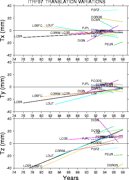
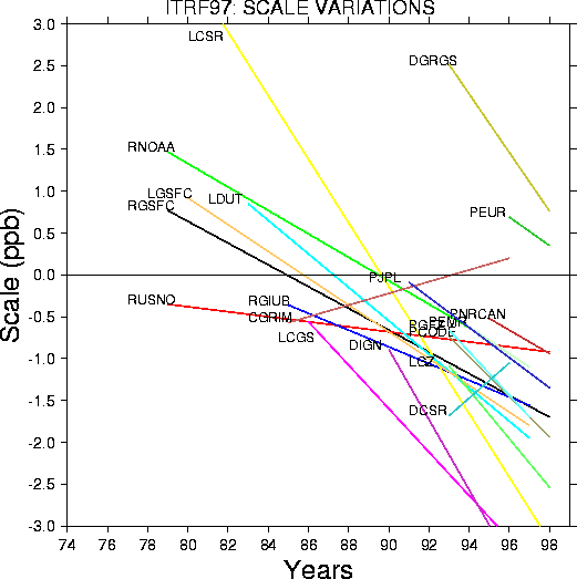
File ITRF97.TSG{.dlLink target=_blank} contains the adjusted transformation parameters at epoch 1997.0 of each individual solution as well as the corresponding rates. The transformation parameters are from each individual solution to the ITRF97 and should be used with the equation ($\fig5$).The rates have to be considered as annual variations to the transformation parameters and should be used with equation ($\fig6$). On the other hand, for a given transformation parameter $T$ provided at an epoch $t_k$, its value at an epoch t in years could be obtained by equation ($\fig7$).
With, $X,Y,Z$ are the coordinates in the ITRF97, and $X_s,Y_s,Z_s$ are the coordinates in the individual system.
Result Analysis
The quality analysis of the ITRF97 results is based more specifically on global residuals per solution ($\tab2$) as well as per site. All residuals on a site-by-site basis resulting from the combination are available in the file ITRF97.RESIDUALS. In this file, the following residuals are provided, per individual solution, for each station within each site, both for positions and velocities:
- ($RX, RY, RZ$) the 3 residual components in the geocentric frame;
- ($RE, RN, RU$) the 3 residual components in the local frame;
- ($NE, NN, NU$) the 3 normalized residual components in the local frame, such as, for example: $ NE = \frac{RE}{\sigma_E}$, where $\sigma_E$ is the uncertainty of the Easting component.
It should be noted that, since the individual solutions were mapped at their Epochs of Minimal Position Variance, this leads obviously to one epoch per station. Consequently, the post fit position residuals are naturally computed at the epoch of each station.
| Solution |
Station nb. |
Position WRMS mm |
Velocity WRMS mm/y |
|---|---|---|---|
| VLBI | |||
| SSC(GSFC) 98 R 01 | 131 | 3.30 | .70 |
| SSC(GIUB) 98 R 01 | 53 | 2.50 | .60 |
| SSC(NOAA) 95 R 01 | 111 | 5.80 | 1.10 |
| SSC(USNO) 98 R 01 | 121 | 2.90 | .60 |
| SLR | |||
| SSC(CGS) 98 L 01 | 75 | 11.90 | 2.20 |
| SSC(CSR) 98 L 01 | 116 | 11.70 | 2.50 |
| SSC(DUT) 98 L 01 | 71 | 19.20 | 3.30 |
| SSC(GSFC) 98 L 01 | 38 | 3.80 | .70 |
| SSC(GZ) 98 L 01 | 50 | 5.20 | 2.80 |
| GPS | |||
| SSC(CODE) 98 P 01 | 130 | 3.70 | 1.60 |
| SSC(EMR) 98 P 01 | 40 | 5.30 | .50 |
| SSC(EUR) 98 P 01 | 47 | 1.90 | 1.80 |
| SSC(GFZ) 98 P 01 | 78 | 8.70 | 2.90 |
| SSC(JPL) 98 P 02 | 64 | 3.60 | 2.20 |
| SSC(NRCAN) 98 P 01 | 117 | 2.10 | 2.80 |
| DORIS | |||
| SSC(CSR) 96 D 01 | 54 | 26.90 | 10.40 |
| SSC(GRGS) 98 D 01 | 61 | 27.90 | 5.50 |
| SSC(IGN) 98 D 04 | 69 | 32.10 | 10.70 |
| Multi-technique | |||
| SSC(GRIM) 98 C 01 | 140 | 10.80 | 4.40 |
